The Complete Engineering Handbook: Data Structures and Algorithms for Production Scalability

Core Philosophy (Why Are We Here?)

You just finished building a fantastic web application. In your local development environment, everything runs at top speed for ten users. Every request processes in milliseconds, and database queries return answers without any delay. But the day you deploy your application to a production server and traffic suddenly spikes to a hundred thousand concurrent requests, disaster strikes. Your server memory and CPU usage hit one hundred percent, API response times stretch into seconds, and eventually, the entire system crashes. Have you ever wondered why code that works perfectly on your local machine breaks down so miserably under real production loads?

There is a widespread misconception in the software engineering industry. Many developers believe that knowing the syntax of a programming language, such as writing loops or conditional statements, is the foundation of software engineering. But in real production environments, simply knowing how to write code is not enough to build scalable systems. When your code executes, you need a deep understanding of how the computer stores data in memory and how the processor handles that information. Without this foundational mechanical knowledge, request bottlenecks are inevitable. It does not matter how powerful your cloud servers or hardware configurations are; inefficient code architecture will destroy your system performance.

What exactly is a data structure? In simple terms, it is the art of organizing and storing data efficiently inside computer memory. To understand this concept, let us look at a real-world analogy. Imagine a disorganized workshop where thousands of tools are scattered randomly across the floor. If you need to find a specific screwdriver in that mess, you will easily waste thirty minutes searching for it. Now, picture a well-organized, smart toolbox where every single tool has a dedicated, custom-fitted slot. With that toolbox, you could grab the exact tool you need in just a few seconds without even looking. A data structure is that smart toolbox for your computer memory, arranging data so that your system can find and process it instantly when needed.

On the other hand, an algorithm is a step-by-step set of logical instructions or a recipe for working with that organized data. You might own the best toolbox in the world, but if you do not know the exact steps required to repair an engine using those tools, you will not get any work done. In the exact same way, simply organizing your data is not enough. You must also choose the fastest logical path to search through, retrieve, or modify that information. The real secret to building high-performing, scalable systems and APIs is the exact combination of the right data structure with an optimized algorithm. Without this powerful pairing, no modern software architecture can truly be production ready.

Performance Measurement Standards (Big-O Notation and Trade-offs)

When we write code or logic as software engineers, measuring how fast that code executes is critical. However, if you try to measure the speed of your code using seconds or milliseconds, you are making a major engineering mistake. Time measurements depend entirely on the processing power of the underlying hardware. A piece of code might run in ten milliseconds on your brand new, high-end laptop, but that exact same code could take a full second to execute on an older device owned by your user. Because of this discrepancy, we need a universal measurement scale that does not rely on hardware specifications or processor speeds. We need a metric that shows how code performance changes as the size of the input data grows.

This universal standard is known as Big-O Notation. It tells us how rapidly the required time or memory will increase as the input data grows in size. In this context, we must evaluate two main concepts: time complexity and space complexity. Time complexity measures how many logical operations or steps the code needs to complete its task. Space complexity measures how much additional memory your code consumes while it runs. Maintaining a clean balance between these two metrics is essential in production architecture. We often have to trade extra memory consumption to gain faster processing speeds, or accept slightly longer processing times to conserve valuable system memory.

Several primary forms of Big-O Notation influence our daily engineering decisions. Here is a simple breakdown of how they work:

• O(1) - Constant Time: This represents peak performance. Whether your system contains ten records or ten million records, this logic will always take the exact same amount of time to execute. For example, grabbing a value directly from an array using its index number does not depend on the size of the dataset.
• O(n) - Linear Time: In this scenario, as the input data multiplies, the execution time multiplies at the exact same rate. If you write a loop to search from the beginning to the end of an array for a specific value, searching through ten million items might require up to ten million iterations.
• O(log n) - Logarithmic Time: This is a highly efficient and fast performance pattern. With this approach, the search area or dataset is cut in half at every single step. Even if the data size doubles, the algorithm only requires one additional step to complete its work. This makes it ideal for working with large databases and sorted lists.
• O(n^2) - Quadratic Time: This is the silent killer of production systems. When you write nested loops in your code, meaning one loop runs inside another loop, the processing time grows geometrically as the data increases. If you have one thousand items, your loop will run one million times, which can instantly freeze your server.

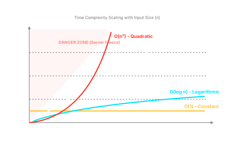Take a look at the diagram above. It clearly shows how performance changes across different Big-O complexities as the input data grows. In production environments, our primary goal is to keep code within constant time or logarithmic time whenever possible, and strictly avoid quadratic time or worse logic at all costs.

Memory Layout and Linear Data Structures (The Foundation)

To truly understand data structures, we first need to look at how computer memory actually works. When you create a variable or store data in your code, the operating system places it in a specific location inside your system memory. You can picture memory as a long, continuous row of billions of tiny boxes. Each box holds one byte of data and has its own unique memory address, much like every house on a street has a unique house number. When the processor wants to read or write data, it communicates directly using that memory address.

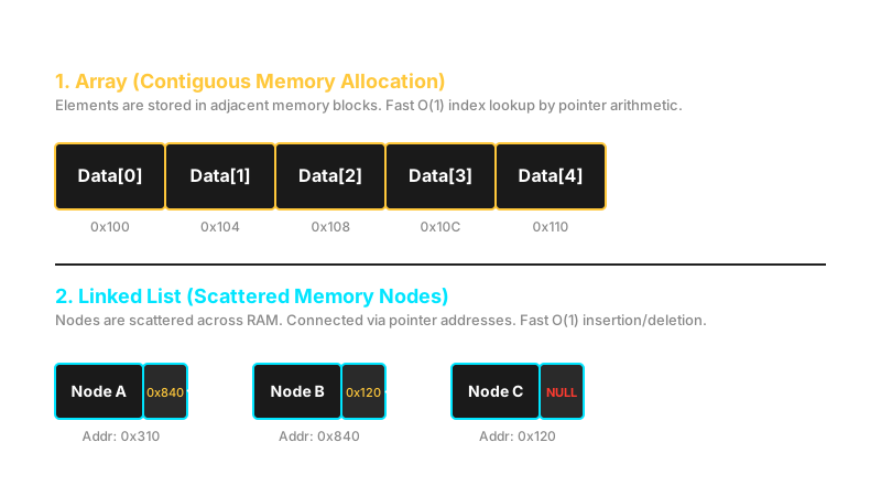
Based on this memory layout, the most fundamental data structure we use is the array. An array is simply a collection of continuous, sequential memory blocks. When you declare an array in your code, the system allocates a continuous strip of memory boxes right next to each other. To picture this, think of booking movie theater tickets with your friends. If you want to sit together and book five seats, the ticketing clerk assigns you five consecutive seats in the exact same row. An array occupies memory in that exact same continuous manner.

Reading data from an array using an index happens in constant time. Because the data items sit right next to each other in memory, the computer uses a simple mathematical formula to calculate the exact memory address of any index instantly. The formula is: $\text{Target Address}=\text{Base Address}+(\text{Index}\times \text{Size of Element})$. However, the major weakness of an array comes into play when you try to insert or delete data from the middle of the sequence. If you want to drop a new item into the middle of an array, you must shift every subsequent item one position to the right to clear space. In an array of ten million items, this shifting process is extremely slow and results in linear time complexity.

To overcome this physical limitation, we use the linked list. In a linked list, data items do not need to sit in continuous, sequential memory blocks like they do in an array. A data block, called a node, can sit anywhere in memory where empty space is available. Every single node contains two things: the actual data value, and a pointer that stores the memory address of the next node in the sequence. To visualize this architecture, think of a classic treasure hunt game. When you find your first clue, it gives you the location of the second clue. You travel to that spot to find the second clue, which then directs you to the third location. A linked list operates on this exact same chaining mechanism.

Deciding whether to use an array or a linked list in production depends entirely on your specific use case. If your system frequently reads data by index number, an array is the best choice. However, if your application constantly inserts and deletes data from the middle of a list and you cannot predict the total data size in advance, a linked list will deliver superior performance. With a linked list, you never have to shift massive amounts of data; you simply update the address stored in the pointers, and the job is done.

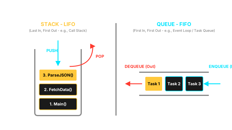
Two other essential concepts in the world of linear data structures are the stack and the queue. A stack operates on a Last-In, First-Out model. A great analogy for a stack is a pile of clean plates sitting on a dining table. When you wash plates and stack them one on top of another, the plate you placed on the very top is always the first one you grab when setting the table for dinner. This architecture is heavily used across software engineering. The back button in your web browser, the call stack during code execution, and the undo and redo features in text editors all rely completely on this stack mechanism.

In contrast, a queue operates on a First-In, First-Out model. A real-world analogy for a queue is a line of people waiting at a bank cashier or a movie theater ticketing counter. The person who arrives first and stands at the front of the line is the first person to receive service and leave the counter. Queues are an indispensable component in backend and systems architecture. The Node.js event loop, background job processing in microservice architectures, and heavy-duty task queues or message brokers like RabbitMQ and Apache Kafka all scale by relying on this exact first-in, first-out principle.

Fastest Data Lookup (Hash Tables and Maps)

When we deal with massive datasets in production engineering, our primary objective is finding specific data as quickly as possible. If you need to search through a database of ten million users to find a specific email address or user profile in just a single millisecond, linear arrays and linked lists simply will not work. For this kind of ultra-fast lookup, an engineer's most powerful weapon is the hash table, also known as a map. A hash table performs the magic of retrieving data from any database or list in constant time, regardless of the dataset size.

The real power behind this lookup speed is the hash function. A hash function is a specialized mathematical algorithm that takes a string, number, or key as input, runs a specific calculation, and converts that key into an integer that serves as a memory index. For example, when you pass the key "user_1029" into a hash table, the hash function uses a mathematical formula to determine that this user profile sits in memory slot number 42. Later, when you request the data for "user_1029" again, the system does not run a search loop; it simply runs the hash function and pulls the data directly from slot 42.

// An example of a simple hash function that converts a string key into an array index
function simpleHash(key: string, arraySize: number): number {
    let hash = 0;
    for (let i = 0; i < key.length; i++) {
        // Performing mathematical calculations using the ASCII code of each character
        hash = (hash + key.charCodeAt(i) * 31) % arraySize;
    }
    return hash;
}

const tableSize = 100;
const index = simpleHash("user_profile_dhaka", tableSize);
console.log(`Data will be stored at index: ${index}`);

However, this brilliant system introduces a major engineering challenge known as a hash collision. Because our system memory and array slots are finite, but the potential number of input keys is infinite, two completely different keys will occasionally generate the exact same memory index. For example, if running the hash calculation on the words "dhaka" and "sylhet" both result in slot number 15, a hash collision occurs. If your system architecture does not handle these collisions with clean logic, you risk system crashes or permanent data loss.

In software architecture, engineers rely on two highly popular and effective techniques to resolve hash collisions:

1. Chaining: In this approach, instead of storing a single data value directly inside each memory slot of the hash table, the slot holds the head of a linked list. Whenever a collision occurs and multiple keys map to the exact same index, the system simply attaches the new data as a new node in that slot's linked list. During a lookup, the hash function locates the correct index first, and then the system runs a brief loop through that tiny linked list to find the exact target data.
2. Open Addressing: This method avoids using linked lists entirely. When the system tries to place new data into a memory slot and discovers that the slot is already occupied, it automatically begins searching for the very next empty slot. To find an open space, it uses techniques like linear probing, which checks slots sequentially one by one, or quadratic probing, which uses mathematical jumps to find empty slots. The new data is then placed into the first empty slot the system discovers.

Non-Linear Structures (The Real Power of Scaling)

So far, every data structure we have discussed, including arrays, linked lists, stacks, and queues, falls under the category of linear data structures. In a linear structure, data items sit in a straight, sequential line. However, many complex real-world problems and massive datasets cannot be modeled efficiently in a simple straight line. When our systems require hierarchical relationships where data elements sit beneath other data elements, we must step into the world of non-linear data structures. The two most important and powerful pillars of this world are trees and graphs.

Trees, and specifically binary search trees, provide an architecture that organizes data in a clear hierarchy. A great analogy for a tree is a corporate organizational chart or a family tree. In a corporate organogram, the Chief Executive Officer sits at the top, directing several vice presidents, who supervise managers, who guide the engineering teams below them. A tree data structure operates in this exact hierarchical format, where the top element is called the root node, and the branching elements below it are called child nodes.

Why do modern relational databases and operating system file systems rely on trees instead of simple arrays? The primary reason is incredible search speed. A binary search tree follows a strict rule: any node placed in the left branch must contain a smaller value, and any node placed in the right branch must contain a larger value. When you search for a specific item, you can determine with absolute certainty at every step whether your target lies to the left or to the right. This simple logic cuts the remaining search space in half with every step, giving us logarithmic time complexity.

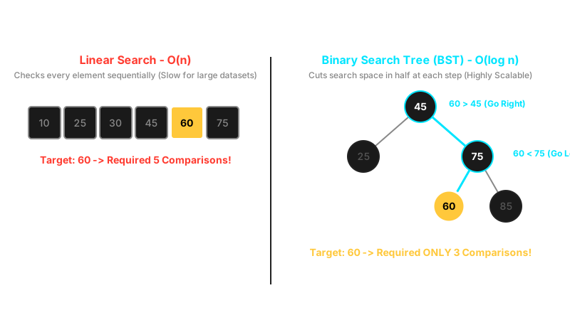In an array of ten million records, a linear search might require ten million loop iterations to find an item located at the very end. In contrast, using a balanced binary search tree, finding any piece of data among those same ten million records requires at most twenty-four to thirty steps. In a production environment, this massive performance difference dictates whether your API responds in milliseconds or crashes from request timeouts.

When we move beyond trees to tackle even more complex, real-world networking logic, we need the graph data structure. A tree is actually just a specialized version of a graph that has a defined root and contains no closed loops or cycles. A graph has no such limitations. A graph consists of two main components: nodes, also called vertices, which represent objects or locations, and edges, which represent the relationship or connection paths between those nodes.

Graphs appear everywhere in real-world software engineering. For example, social media friend networks on platforms like Facebook or LinkedIn are massive graphs. Every user is a node, and a friendship connection between two users represents an edge. When the system calculates mutual friends or suggests connections, graph traversal algorithms run in the backend. Similarly, ride-sharing applications and mapping platforms like Google Maps or Uber store entire city road networks in memory as graphs. Street intersections act as nodes, and the roads connecting them act as edges. To calculate the shortest and fastest route between two locations, these systems use specialized graph algorithms like Dijkstra or A-star. Even internet data routing protocols rely entirely on graph architectures to move data packets across the globe efficiently.

Core Algorithmic Techniques and Paradigms

Once we have organized our data cleanly in memory, our next step is executing various operations and logical tasks on that data. To do this effectively, we need to master a core set of algorithmic techniques and problem-solving paradigms. In daily software engineering, the two most common computational tasks we face are searching and sorting.

We have already seen that linear search is a slow approach where a loop checks items one by one, resulting in linear time complexity. However, if your dataset is already sorted in ascending order, you can use binary search. This powerful algorithm compares your target value with the middle item of the dataset and eliminates half of the remaining items in a single bound. This allows you to find any data point in logarithmic time.

Now let us examine sorting. Keeping data sorted is essential in production systems because binary search and ultra-fast database queries are impossible without sorted data. While simple sorting algorithms work fine for small lists, sorting millions of database records requires advanced algorithms. The two most widely used production sorting algorithms are QuickSort and MergeSort.

• QuickSort: This is a divide-and-conquer algorithm. It selects a specific item from the dataset to act as a pivot, and then shifts all smaller values to the left of the pivot and all larger values to the right. It then recursively sorts the left and right sections using the same method. Its average time complexity is O(n log n), and it uses very little additional memory space. However, if the data is already sorted in reverse order and the algorithm chooses a poor pivot, its worst-case performance can drop to quadratic time.
• MergeSort: This algorithm also relies on the divide-and-conquer paradigm. It continually cuts the entire dataset in half until each smaller subsection contains only a single item. It then merges those individual items back together in sequential order to produce a fully sorted list. Its biggest advantage is reliability: regardless of how messy the initial data is, MergeSort is guaranteed to complete its work in O(n log n) time. The trade-off is space complexity; merging the lists requires allocating additional memory space equal to O(n).

How should we think when facing a new or complex engineering problem? In software architecture, we generally rely on three major problem-solving paradigms:

1. Brute Force: This is the most straightforward problem-solving approach, without any clever optimizations. Using brute force, your code checks every single possible solution or path one by one until it finds the correct answer. While this approach is easy to code and guaranteed to find the right answer, it is extremely slow in production systems, often resulting in time complexities of O(n^2) or even exponential time, O(2^n).
2. Greedy Algorithm: With this mindset, the algorithm makes whatever decision looks best and most profitable at the exact current moment, without considering future consequences or the big picture. It chooses a locally optimal step at each stage with the hope of reaching a globally optimal solution. For example, when routing network packets at the lowest cost, choosing the shortest available path at every single router junction follows greedy logic. While this approach executes very quickly, it does not guarantee a one-hundred-percent optimal solution for every type of problem.
3. Dynamic Programming: This is a highly sophisticated and intelligent engineering paradigm. When you can break a massive, complex problem down into many smaller, overlapping subproblems, dynamic programming is the right tool for the job. Its core philosophy is simple: never repeat a calculation you have already completed. The system solves the smaller problems once and stores those answers inside a memory map or array, a technique known as memoization or caching. When the algorithm encounters the exact same calculation later, it bypasses processing and reads the result directly from memory. Because of this caching mechanism, problems that would take brute force thousands of years to solve can be resolved in just a few seconds using dynamic programming.

Production Engineering and Real-World Use Cases

After covering the theoretical foundations, let us see how we apply this knowledge of data structures and algorithms directly to daily production engineering and real-world systems. We will examine two vital production use cases in detail: database indexing and caching architecture.

First, let us discuss database indexing. When you work with a relational database like MySQL or PostgreSQL storing millions of user records, how does a query like SELECT * FROM users WHERE email = 'example@test.com' return an answer in just a few milliseconds? If you have not created an index on the email column, the database engine must read every single record from the hard disk or solid-state drive into memory one by one to check for a match. This is called a full table scan. If high traffic hits your system while the database performs full table scans across ten million records, your server processor and memory will overload instantly, causing the database to crash.

To resolve this bottleneck, database engines use specialized balanced tree structures known as B-Trees and B+ Trees. When you create an index on a specific column, the database organizes that data into a B+ Tree and stores it in a dedicated space in memory or on disk. The defining feature of a B+ Tree is that every single node can hold multiple data values and many child pointers, which keeps the overall height of the tree extremely low. As a result, finding a specific record among tens of millions of entries requires the database to execute only three or four disk read operations, guaranteeing logarithmic performance.

Our second production use case is caching architecture. In any high-traffic, scalable system, we use caching layers like Redis or Memcached to reduce the database load and serve instant responses to users. However, memory space in RAM is extremely limited and expensive. Therefore, we must design a smart caching architecture that retains the most frequently needed data in memory while automatically removing old or unused items when memory fills up. The industry-standard algorithm for this requirement is the Least Recently Used cache, commonly known as an LRU Cache.

To build a production-grade LRU cache, we need an architecture where two specific operations occur in constant time:

1. Looking up data using any key.
2. Updating memory during data insertion or when removing old items.

Using only an array or only a linked list cannot achieve this. Instead, software architects combine two distinct structures: a hash map and a doubly linked list. The hash map guarantees constant time data lookups, while the doubly linked list allows us to add or remove nodes from any position in constant time without shifting data.

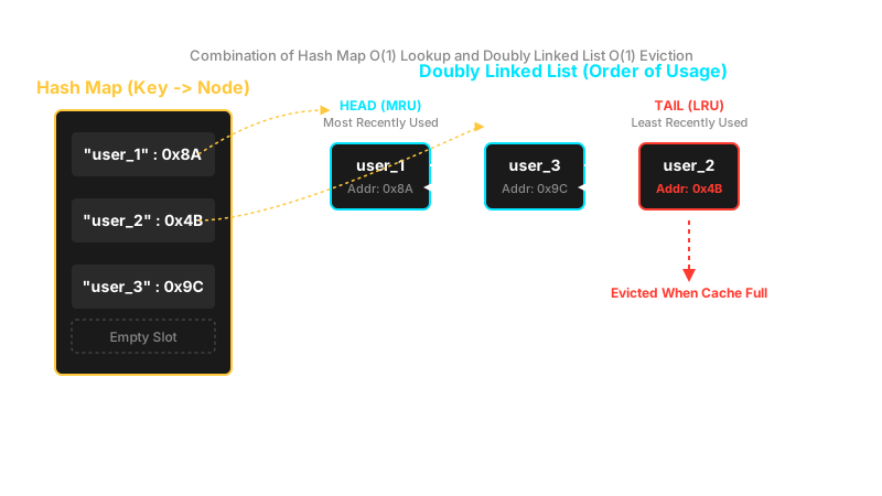
Consider the architecture involved here. Each key in the hash map points directly to the memory address of a specific node inside the doubly linked list. Whenever an item is read or written, the system moves that node to the very front of the doubly linked list, marking it as the most recently used item. When the cache hits its maximum capacity, the system targets the node sitting at the very end of the list, marking it as the least recently used item, and removes it from memory in constant time.

Here is a production-ready, fully type-safe TypeScript implementation that combines a hash map and a doubly linked list to create a functioning LRU cache:

// Architecture of each node in the doubly linked list
class CacheNode<K, V> {
    public key: K;
    public value: V;
    public prev: CacheNode<K, V> | null = null;
    public next: CacheNode<K, V> | null = null;

    constructor(key: K, value: V) {
        this.key = key;
        this.value = value;
    }
}

// Complete LRU Cache implementation
export class LRUCache<K, V> {
    private capacity: number;
    private cacheMap: Map<K, CacheNode<K, V>>;
    private head: CacheNode<K, V>;
    private tail: CacheNode<K, V>;

    constructor(capacity: number) {
        this.capacity = capacity;
        this.cacheMap = new Map();

        // Creating dummy head and tail nodes to make edge case handling easier
        this.head = new CacheNode<K, V>({} as K, {} as V);
        this.tail = new CacheNode<K, V>({} as K, {} as V);
        this.head.next = this.tail;
        this.tail.prev = this.head;
    }

    // Constant time logic to disconnect any node from the linked list
    private removeNode(node: CacheNode<K, V>): void {
        const prevNode = node.prev;
        const nextNode = node.next;

        if (prevNode && nextNode) {
            prevNode.next = nextNode;
            nextNode.prev = prevNode;
        }
    }

    // Constant time logic to add any node right after the head
    private addToHead(node: CacheNode<K, V>): void {
        node.prev = this.head;
        node.next = this.head.next;

        if (this.head.next) {
            this.head.next.prev = node;
        }
        this.head.next = node;
    }

    // Constant time read method
    public get(key: K): V | null {
        if (!this.cacheMap.has(key)) {
            return null;
        }

        const node = this.cacheMap.get(key)!;
        // Since this data was just accessed, move it to the head
        this.removeNode(node);
        this.addToHead(node);

        return node.value;
    }

    // Constant time write method
    public put(key: K, value: V): void {
        if (this.cacheMap.has(key)) {
            // If data already exists, update its value and move it to the head
            const existingNode = this.cacheMap.get(key)!;
            existingNode.value = value;
            this.removeNode(existingNode);
            this.addToHead(existingNode);
        } else {
            // Creating a new node for new data
            const newNode = new CacheNode(key, value);
            this.cacheMap.set(key, newNode);
            this.addToHead(newNode);

            // If capacity is exceeded, remove the oldest data (the node right before the tail)
            if (this.cacheMap.size > this.capacity) {
                const lruNode = this.tail.prev;
                if (lruNode && lruNode !== this.head) {
                    this.removeNode(lruNode);
                    this.cacheMap.delete(lruNode.key);
                }
            }
        }
    }
}

// Production test execution
const userCache = new LRUCache<string, string>(2);
userCache.put("user_1", "Alice Profile");
userCache.put("user_2", "Bob Profile");

console.log(userCache.get("user_1")); // Alice Profile (user_1 is now the most recently used)

// Inserting new data exceeds capacity, evicting user_2 (least recently used) from memory
userCache.put("user_3", "Charlie Profile");
console.log(userCache.get("user_2")); // null (the data has been evicted from the cache)

Recap and Production Checklist

Through this detailed exploration of systems architecture, one core lesson becomes clear: the primary difference between a junior developer and an experienced system architect lies in their depth of thinking. Junior developers focus on whether their code runs and produces the correct output. System architects focus on what happens when that code executes ten million times across distributed networks, evaluating memory layouts, network latency, and processor loads. Data structures and algorithms are not just theoretical trivia meant for passing coding interviews; they form the absolute bedrock of your software engineering career, giving you the power to design fast, scalable, and reliable production systems.

The next time you design a new system architecture or tackle a complex performance bottleneck, keep this developer decision checklist in mind:

• Use an Array when: Your data size is fixed and known in advance, you need maximum memory optimization, and your system frequently reads elements by their index numbers in constant time.
• Use a Linked List when: Your data size changes constantly during runtime, and your application needs to insert or delete items from the beginning or middle of the sequence without delay.
• Use a Hash Table or Map when: You need to look up data instantly using a specific key from a massive dataset in constant time.
• Use a Tree or Binary Search Tree when: Your data naturally forms a hierarchical structure, and you need to execute fast range queries or searches across sorted records.
• Use a Graph when: You need to model complex networking logic, social media connections, mapping and routing systems, or real-world relationship paths.
• Use a Queue when: Your system needs to process incoming requests, background tasks, or worker jobs sequentially in a First-In, First-Out order.
• Use a Stack when: Your logic requires a Last-In, First-Out architecture, such as parsing programming syntax, tracking execution history, or building undo and redo mechanisms.

Best of luck on your engineering journey. By making the right architectural decisions, may every system you build be completely production ready and highly scalable.